PRISMA flow diagrams with ggconsort • ggconsort

PRISMA flow diagrams document the flow of records through a systematic review, from identification through screening to the final set of included studies. Structurally they are close cousins of CONSORT diagrams, so the same two-stage ggconsort workflow applies: count cohorts while you wrangle the citation data, then lay out boxes and arrows.

This article builds a diagram in the style of the PRISMA 2020 statement for a hypothetical systematic review.

Citation data

In a real review, you would start from a data frame of citation records exported from your reference manager, with one row per record and columns that track each record’s fate. Here we simulate one.

library(ggconsort)
library(dplyr)

citations <- tibble(id = 1:500) |>
  mutate(
    source = if_else(id <= 412, "Databases", "Registers"),
    duplicate = id <= 102,
    passed_screen = !duplicate & id > 353,
    retrieved = passed_screen & id > 362,
    exclusion_reason = case_when(
      retrieved & id <= 409 ~ "Wrong population",
      retrieved & id <= 448 ~ "Wrong outcome",
      retrieved & id <= 469 ~ "Wrong study design",
      TRUE ~ NA_character_
    )
  )

head(citations)
#> # A tibble: 6 × 6
#>      id source    duplicate passed_screen retrieved exclusion_reason
#>   <int> <chr>     <lgl>     <lgl>         <lgl>     <chr>           
#> 1     1 Databases TRUE      FALSE         FALSE     NA              
#> 2     2 Databases TRUE      FALSE         FALSE     NA              
#> 3     3 Databases TRUE      FALSE         FALSE     NA              
#> 4     4 Databases TRUE      FALSE         FALSE     NA              
#> 5     5 Databases TRUE      FALSE         FALSE     NA              
#> 6     6 Databases TRUE      FALSE         FALSE     NA

Stage 1: count the cohorts

Each PRISMA box is a cohort. As in a CONSORT workflow, cohort_define() derives each cohort from the full set of records or from a previously defined cohort, and anti_join() is a convenient way to count the records that drop out at each step.

review_cohorts <-
  citations |>
  cohort_start("Records identified") |>
  cohort_define(
    from_databases = .full |> filter(source == "Databases"),
    from_registers = .full |> filter(source == "Registers"),
    screened = .full |> filter(!duplicate),
    duplicates = anti_join(.full, screened, by = "id"),
    sought = screened |> filter(passed_screen),
    screened_out = anti_join(screened, sought, by = "id"),
    assessed = sought |> filter(retrieved),
    not_retrieved = anti_join(sought, assessed, by = "id"),
    included = assessed |> filter(is.na(exclusion_reason)),
    excluded_population = assessed |> filter(exclusion_reason == "Wrong population"),
    excluded_outcome = assessed |> filter(exclusion_reason == "Wrong outcome"),
    excluded_design = assessed |> filter(exclusion_reason == "Wrong study design")
  ) |>
  cohort_label(
    from_databases = "Databases",
    from_registers = "Registers",
    screened = "Records screened",
    duplicates = "Duplicate records removed",
    sought = "Reports sought for retrieval",
    screened_out = "Records excluded",
    assessed = "Reports assessed for eligibility",
    not_retrieved = "Reports not retrieved",
    included = "Studies included in review",
    excluded_population = "Wrong population",
    excluded_outcome = "Wrong outcome",
    excluded_design = "Wrong study design"
  )

review_cohorts
#> A ggconsort cohort of 500 observations with 12 cohorts:
#>   - from_databases (412)
#>   - from_registers (88)
#>   - screened (398)
#>   - duplicates (102)
#>   - sought (147)
#>   - screened_out (251)
#>   - assessed (138)
#>   - not_retrieved (9)
#>   ...and 4 more.

Stage 2: lay out the diagram

Each PRISMA box declares a row and col grid position: the main flow runs down the "main" column, with the reasons for attrition beside it in the "side" column. A box named after a cohort labels itself with that cohort’s label and count, so the single-count boxes need nothing but a name and a position; custom multi-line labels are built with <br> (labels are rendered by gridtext, so markdown and HTML formatting work). Arrows connect boxes by name — boxes in the same column are joined vertically and boxes in the same row horizontally, PRISMA-style, from box edge to box edge.

The furniture of the official template is a few consort_stage_add() calls: the rotated stage labels sit in the left margin (the default column), with row = c(2, 4) centering “Screening” across those rows, and the header bar spans both columns via col = c("main", "side") in the template’s amber.

ggconsort measures every box when the plot is drawn and computes the spacing to fit the figure, so no coordinates are needed anywhere; equal_columns = TRUE matches the uniform box widths of the official template.

review_prisma <- review_cohorts |>
  consort_box_add(
    "identified", row = 1, label = glue::glue(
      "Records identified from:<br>
      {cohort_count_adorn(review_cohorts, from_databases)}<br>
      {cohort_count_adorn(review_cohorts, from_registers)}"
    )
  ) |>
  consort_box_add(
    "duplicates", row = 1, col = "side", label = glue::glue(
      "Records removed before screening:<br>
      {cohort_count_adorn(review_cohorts, duplicates)}"
    )
  ) |>
  consort_box_add("screened", row = 2) |>
  consort_box_add("screened_out", row = 2, col = "side") |>
  consort_box_add("sought", row = 3) |>
  consort_box_add("not_retrieved", row = 3, col = "side") |>
  consort_box_add("assessed", row = 4) |>
  consort_box_add(
    "excluded", row = 4, col = "side", label = glue::glue(
      "Reports excluded:<br>
      • {cohort_count_adorn(review_cohorts, excluded_population)}<br>
      • {cohort_count_adorn(review_cohorts, excluded_outcome)}<br>
      • {cohort_count_adorn(review_cohorts, excluded_design)}"
    )
  ) |>
  consort_box_add("included", row = 5) |>
  consort_arrow_add(start = "identified", end = "screened") |>
  consort_arrow_add(start = "screened", end = "sought") |>
  consort_arrow_add(start = "sought", end = "assessed") |>
  consort_arrow_add(start = "assessed", end = "included") |>
  consort_arrow_add(start = "identified", end = "duplicates") |>
  consort_arrow_add(start = "screened", end = "screened_out") |>
  consort_arrow_add(start = "sought", end = "not_retrieved") |>
  consort_arrow_add(start = "assessed", end = "excluded") |>
  consort_stage_add(
    "Identification of studies via databases and registers",
    row = 0, col = c("main", "side"), fill = "#ffc000"
  ) |>
  consort_stage_add("Identification", row = 1, angle = 90) |>
  consort_stage_add("Screening", row = c(2, 4), angle = 90) |>
  consort_stage_add("Included", row = 5, angle = 90)

library(ggplot2)

review_prisma |>
  ggplot() +
  geom_consort(equal_columns = TRUE) +
  theme_consort()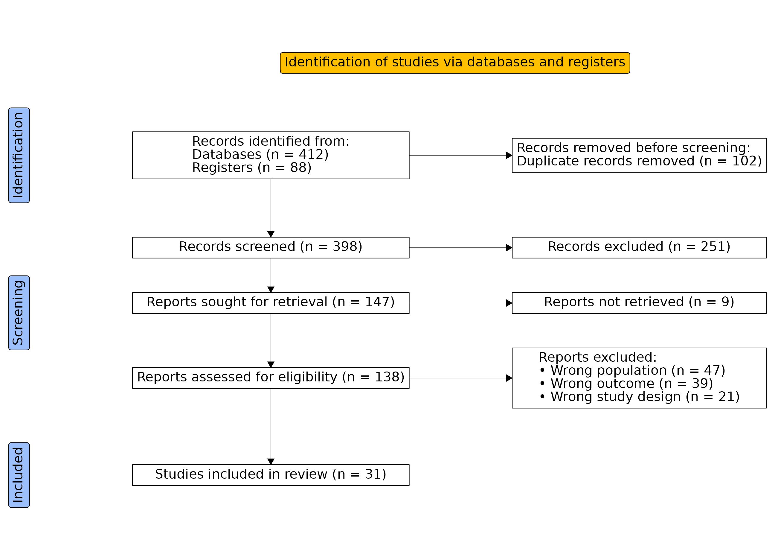

PRISMA 2020 flow diagram: 500 records identified from databases and registers, 398 screened after removing 102 duplicates, 147 reports sought, 138 assessed for eligibility, and 31 studies included in the review

At analysis time, the included studies are one cohort_pull() away:

review_cohorts |>
  cohort_pull(included)
#> # A tibble: 31 × 6
#>       id source    duplicate passed_screen retrieved exclusion_reason
#>    <int> <chr>     <lgl>     <lgl>         <lgl>     <chr>           
#>  1   470 Registers FALSE     TRUE          TRUE      NA              
#>  2   471 Registers FALSE     TRUE          TRUE      NA              
#>  3   472 Registers FALSE     TRUE          TRUE      NA              
#>  4   473 Registers FALSE     TRUE          TRUE      NA              
#>  5   474 Registers FALSE     TRUE          TRUE      NA              
#>  6   475 Registers FALSE     TRUE          TRUE      NA              
#>  7   476 Registers FALSE     TRUE          TRUE      NA              
#>  8   477 Registers FALSE     TRUE          TRUE      NA              
#>  9   478 Registers FALSE     TRUE          TRUE      NA              
#> 10   479 Registers FALSE     TRUE          TRUE      NA              
#> # ℹ 21 more rows